pyinfluence

Training data attribution for scikit-learn estimators.

pyinfluence answers two questions about a fitted scikit-learn model. Per-test-point: which training examples raised or lowered the model's loss or prediction at each test point, returned as a matrix of scores with one entry per test-point/training-example pair. Per-functional: how much each training example moves any scalar property of the model (a fairness gap, AUROC, worst-group loss, or a functional you define), estimated as the effect of removing that example and refitting. It targets scientific workflows that need per-example diagnostics (dataset debugging, auditing, sensitivity analysis), not end-user-facing explanations.

You want to know	Reach for
Which training points drive this prediction or its loss?	influence() one-shot; InfluenceFunctions, LOOInfluence, BanzhafInfluence, BootstrapInfluence
Which training points drive a scalar property (gap, AUROC, ...)?	FunctionalInfluence + builders in pyinfluence.functionals
Which training points drive a fairness disparity?	pyinfluence.fairness.disparity + the same engine
Are these scores real?	removal_curve, RefitFunctionalInfluence (exact ground truth), stability_replicates, pyinfluence.viz

Installation

pip install pyinfluence

To install the latest development version from GitHub:

pip install git+https://github.com/maschulz/pyinfluence

Optional plotting utilities:

pip install "pyinfluence[viz]"

Quickstart

from sklearn.datasets import make_regression
from sklearn.linear_model import Ridge
from sklearn.model_selection import train_test_split

from pyinfluence import influence, top_influential

X, y = make_regression(n_samples=200, n_features=10, noise=0.1, random_state=0)
X_train, X_test, y_train, y_test = train_test_split(X, y, test_size=0.2, random_state=0)

model = Ridge(alpha=1.0).fit(X_train, y_train)

# scores has shape (n_test, n_train)
scores = influence(model, X_train, y_train, X_test, y_test, method="auto", mode="loss")

helpful_idx, harmful_idx = top_influential(scores[0], k=5)
print("Most helpful training indices:", helpful_idx)
print("Most harmful training indices:", harmful_idx)

If you will explain multiple test sets, request the fitted attributor:

scores, attr = influence(
    model,
    X_train, y_train,
    X_test, y_test,
    method="auto",
    mode="loss",
    return_attributor=True,
)
scores2 = attr.explain(X_test[:5], y_test[:5])

What is being estimated?

Notation

• Training set $D = {z_j}_{j=1}^n$, with $z_j = (x_j, y_j)$.
• Test inputs $X_{\mathrm{test}} = {x_i}_{i=1}^m$.
• Influence matrix $S \in \mathbb{R}^{m \times n}$, where $S_{ij}$ refers to training point $j$ and test point $i$. Every attributor's explain returns scores with this (n_test, n_train) shape and indexing.

Modes

All attributors support mode="loss" and mode="prediction", but classification prediction mode is method-dependent.

• Loss mode (mode="loss", default):

  • Estimates how a training point affects test loss.
  • Requires y_test for all methods.
  • Intended interpretation: positive values indicate training points that are helpful for reducing loss at the test point.

• Prediction mode (mode="prediction"):

  • Regression: influence on the scalar prediction $f(x)$. Does not require y_test.
  • Classification:
    • LOOInfluence, BanzhafInfluence, BootstrapInfluence: influence on the true-class score at $x$, so requires y_test to identify the true class.
    • InfluenceFunctions (binary only): influence on the model’s positive-class probability $P_\theta(Y=1 \mid x)$ when available, and otherwise on a linear decision value (e.g., for RidgeClassifier). It does not require y_test.

Sign convention in loss mode

Loss-mode signs are aligned to a removal interpretation (and validated by tests):

• $S_{ij} > 0$: training point $j$ is helpful for test point $i$; removing $z_j$ increases test loss.
• $S_{ij} < 0$: training point $j$ is harmful for test point $i$; removing $z_j$ decreases test loss.

Worked examples

1) Self-influence as an outlier/mislabel heuristic

import numpy as np
from sklearn.linear_model import Ridge

from pyinfluence import InfluenceFunctions, self_influence, find_mislabeled

model = Ridge(alpha=1.0).fit(X_train, y_train)
attr = InfluenceFunctions(mode="loss", damping=1e-5).fit(model, X_train, y_train)

s_self = self_influence(attr)
suspected = find_mislabeled(attr, threshold="auto")

print("Largest |self-influence| indices:", np.argsort(np.abs(s_self))[-10:][::-1])
print("Suspected mislabeled indices:", suspected[:10])

Interpretation: find_mislabeled is a ranking heuristic (z-scores of absolute self-influence); it is not a proof of label error, and its 'auto' threshold is deliberately conservative. For triage under an inspection budget, rank by np.abs(self_influence(attr)) and take your top-k instead. Self-influence measures atypicality: plain per-sample training loss is an equally strong baseline, corrupted features (as opposed to labels) leave a trace it does not read, and detection degrades sharply for plausible, near-boundary errors. Validate on your data with an injection experiment (viz.plot_detection_curve) before trusting the ranking.

2) Explaining a single (mis)prediction

The most common interactive workflow: pick a test case, ask which training points drove it, and say how sure you are.

import numpy as np
from pyinfluence import InfluenceFunctions, LOOInfluence, stability_replicates
from pyinfluence import compare_attributors, viz

attr = InfluenceFunctions(mode="loss", damping=1e-5).fit(model, X_train, y_train)
i = int(np.argmax(np.abs(model.predict(X_test) - y_test)))   # worst test case

scores = attr.explain(X_test[[i]], y_test[[i]])
viz.plot_top_influencers(scores, k=8)                        # who drove it

# how sure are we? (1) slow method agrees, (2) ranking survives resampling
stats = compare_attributors(attr, LOOInfluence(mode="loss", verbose=0).fit(
    model, X_train, y_train), X_test[[i]], y_test[[i]])
reps = stability_replicates(attr, X_test[[i]], y_test[[i]], n_replicates=20)
viz.plot_top_k_stability(reps, k=8)

fig = viz.report(attr, X_test, y_test)   # returns a bare Figure (no axes)

Section 4 of examples/showcase.ipynb walks through this end to end.

3) Comparing methods on the same problem

import numpy as np
from pyinfluence import InfluenceFunctions, LOOInfluence, compare_attributors

attr_if = InfluenceFunctions(mode="loss", damping=1e-5).fit(model, X_train, y_train)
attr_loo = LOOInfluence(mode="loss", n_jobs=-1, verbose=0).fit(model, X_train, y_train)

stats = compare_attributors(attr_if, attr_loo, X_test, y_test, k=10)
print(stats)  # pearson/spearman/kendall + top_k_overlap

scores_if = attr_if.explain(X_test, y_test)
scores_loo = attr_loo.explain(X_test, y_test)
print("Correlation:", np.corrcoef(scores_if.ravel(), scores_loo.ravel())[0, 1])

Per-test-point attribution methods

All methods share the same interface:

attr.fit(model, X_train, y_train)
scores = attr.explain(X_test, y_test)  # shape (n_test, n_train)

Influence functions (InfluenceFunctions)

InfluenceFunctions implements the classical influence-function approximation for smooth empirical risk minimization, specialized to closed-form Hessians for specific scikit-learn estimators.

For a scalar per-example loss $\ell(z;\theta)$, scores are the removal-calibrated influence-function quantity

$$ S_{ij} ;=; \frac{1}{n},\nabla_\theta \ell(z_i^{\mathrm{test}};\theta)^\top , H_\theta^{-1} , \nabla_\theta \ell(z_j;\theta), $$

with

$$ H_\theta ;=; \frac{1}{n}\sum_{k=1}^n \nabla_\theta^2 \ell(z_k;\theta) ;+; \lambda I , $$

where $\lambda$ is the model's L2 regularization expressed in the per-sample-average objective ($\alpha/n$ for Ridge-family models, $1/(Cn)$ for LogisticRegression; the intercept dimension is not regularized). For KernelRidge the dual-space penalty matrix is $(\lambda/n)K$, which makes the formula exact at the KRR stationarity condition.

The $1/n$ factor calibrates the classical infinitesimal-upweighting derivative to the finite effect of deleting one training point (a weight change of $-1/n$), so InfluenceFunctions scores estimate the same quantity as LOOInfluence, in both sign and magnitude. Agreement with exact leave-one-out retraining (correlation and regression slope ≈ 1) is tested in this repository (tests/test_loo_agreement.py). The slope claim assumes the leave-one-out refit preserves the per-sample-average regularization (alpha scaled by (n−1)/n); a naive refit at fixed alpha shifts the effective regularization and can show a different slope at small n. See the test file for the exact protocol.

Supported estimators (as implemented):

• sklearn.linear_model.Ridge, RidgeCV
• sklearn.linear_model.LinearRegression
• sklearn.linear_model.LogisticRegression, LogisticRegressionCV (binary only)
• sklearn.linear_model.RidgeClassifier, RidgeClassifierCV (binary only)
• sklearn.kernel_ridge.KernelRidge (dual-space influence functions; the Hessian is n_train x n_train)

Stability parameter:

• damping: a diagonal term added to the Hessian for numerical stability. Larger values typically reduce influence magnitudes and can reduce numerical instability on ill-conditioned problems.

Leave-one-out retraining (LOOInfluence)

LOOInfluence refits the estimator once per training point (excluding that point) and measures the resulting change in loss or prediction:

• Loss mode: $S_{ij} = L_i(D \setminus {z_j}) - L_i(D)$.
• Prediction mode (regression): $S_{ij} = f_i(D) - f_i(D \setminus {z_j})$.
• Prediction mode (classification): uses the true-class score, so requires y_test.

This method is model-agnostic but computationally expensive. For classifiers, refits can fail after deletion (e.g., a class disappears); in that case the corresponding scores are NaN.

Data Banzhaf (BanzhafInfluence)

BanzhafInfluence estimates an average marginal contribution using Monte Carlo subset sampling. For each training point, it samples subsets S of the remaining points (each included independently with probability 1/2), then refits models on S with and without the point:

• Loss mode: $S_{ij} \approx \mathbb{E}_S\left[ L_i(S) - L_i(S \cup {z_j}) \right]$ (positive indicates the point reduces loss on average).
• Prediction mode: analogous, with the value-at-test being a prediction (regression) or true-class score (classification).

This construction satisfies symmetry and null-player properties up to Monte Carlo error. It does not enforce Shapley efficiency.

Bootstrap out-of-bag (BootstrapInfluence)

BootstrapInfluence fits n_estimators bootstrap models and uses out-of-bag (OOB) runs to approximate a point's contribution: for each training point, it compares the mean test value across runs where the point is out-of-bag to the mean across runs where it is in-bag. Both sides use roughly 63% of the data, so the comparison isolates the point's presence.

OOB counts can be small (or zero) for some points when n_estimators is small; in that case scores may be noisy or NaN.

Choosing a method

• If your model is supported by InfluenceFunctions and you need fast, deterministic estimates: start there.
• If you need model-agnostic influence and the training set is small enough to refit many times: use LOOInfluence.
• If you want a subset-average notion of contribution (data valuation) and can afford repeated refits: use BanzhafInfluence.
• If you want a model-agnostic baseline with controllable compute and are comfortable with OOB variability: use BootstrapInfluence.
• Non-linear models (trees, boosting, nets): the model-agnostic estimators measure different estimands (full-data LOO effect vs. subset-averaged effects) and can rank points almost independently of one another on highly non-linear models. We have observed per-point correlations near 0 between LOOInfluence and BootstrapInfluence on boosted trees, with each still beating the random baseline on its own removal_curve. Aggregate validity does not imply per-point identifiability: run compare_attributors between two methods and a removal_curve before acting on any individual ranking.

High-level API: influence(...)

pyinfluence.influence() provides a one-shot interface that selects an attributor:

• method="auto" uses InfluenceFunctions for supported linear(-like) models (including binary classifiers and KernelRidge).
• otherwise, or if unsupported: uses fallback (default bootstrap; alternatives loo or banzhaf).

from pyinfluence import influence

scores = influence(
    model,
    X_train, y_train,
    X_test, y_test,
    method="auto",
    fallback="bootstrap",
    mode="loss",
)

Utilities

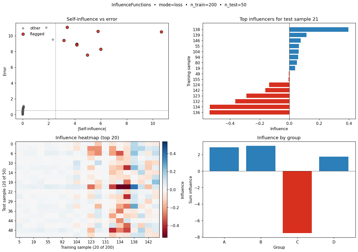
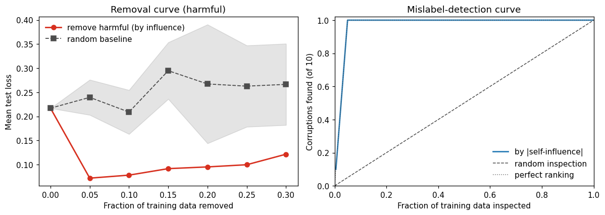
• top_influential(scores, k=10): indices of most helpful / most harmful training points.
• self_influence(attributor, ...): diagonal of the influence matrix, each training point explained against itself. Uses a direct-diagonal fast path (O(n) memory) for InfluenceFunctions, LOOInfluence, and BootstrapInfluence.
• influence_summary(scores, ...): summary statistics (mean/std/percentiles/sparsity/NaN count).
• find_mislabeled(attributor, threshold="auto"): flags outliers based on z-scores of absolute self-influence (heuristic).
• compare_attributors(attr1, attr2, ...): correlations and top-k overlap across two methods.
• aggregate_influence(scores, axis=0, method=...): aggregate across test points or train points.
• influence_by_group(scores, groups, ...): aggregate influence by group labels on training samples.
• removal_curve(attributor, X_test, y_test, ...): retrain after dropping the top-k% most harmful (or helpful) training points and compare to a random-removal baseline, the standard validation of whether influence scores carry signal. Requires mode='loss'; see help(removal_curve) for the fractions/direction/n_random parameters and the returned dict.
• stability_replicates(attributor, X_test, y_test, n_replicates=20): rerun the attributor on bootstrap-resampled training sets; feeds viz.plot_top_k_stability. This measures a different uncertainty than scores_std_ (Banzhaf/Bootstrap): per-score Monte-Carlo noise given the training set vs. ranking stability under training-data resampling. The two can disagree, so check both. Cost is n_replicates full attributor refits (independent of test-set size).
• supports(model): (True, None) if InfluenceFunctions can handle the fitted model, else (False, reason); never raises or warns.

NaN policy. Refit-based attributors produce NaN where a point's effect is unmeasurable (failed refits, no OOB runs), with a warning naming the affected points. All utilities and plots then exclude NaN from rankings and statistics (again with a warning); NaN is never silently ranked, averaged, or treated as zero.

Functional influence: attribute any scalar property of the model

Beyond per-test-point scores, pyinfluence attributes scalar functionals F(θ) (any quantity defined through the model's per-sample scores or losses on a fixed reference set) to training examples: scores[j] ≈ F(D \ z_j) − F(D).

Three estimators share the estimand: FunctionalInfluence (closed form for supported GLMs; hessian="identity" gives the gradient-dot baseline), RefitFunctionalInfluence (exact leave-one-out ground truth, model-agnostic), and SubsampledFunctionalInfluence (Monte-Carlo subsets, model-agnostic). A Functional bundles the function with an optional analytic gradient and the value kind; bare callables fn(scores, y) -> float work too (differentiated by finite differences). Non-smooth functionals (rank statistics like AUROC, marked differentiable=False) are attributed by perturbation evaluation: the closed form linearizes each removal's parameter step as usual, then evaluates the exact functional on the perturbed scores, so no smoothing or temperature is ever needed. The refit-based estimators evaluate any functional directly regardless. One fitted attributor can explain any number of functionals (explain(..., functional=...)), and functional_value(model, X, F, y) evaluates one directly.

Ready-made builders live in pyinfluence.functionals, domain-neutral, all with analytic gradients:

Builder	Functional
mean(of)	average score or loss on the reference set
group_gap(groups, keep=None, of)	difference in group means, optionally label-conditioned
cohens_d(groups)	standardized group gap (pooled-SD normalized)
worst_group_mean(groups, of)	max over groups of the group mean
auroc(pos_label)	ranking quality: the exact Mann–Whitney AUROC. Attributed by perturbation evaluation (below). It preserves the estimand's quantization (removals that swap no pair score exactly 0); the perturbation approximation matches exact-refit ground truth at r > 0.99 on the package benchmark, but is dataset-dependent — on small or high-leverage problems the per-point correlation can be much lower, so validate against RefitFunctionalInfluence on your data.

All builders (and fitted attributors holding them) are picklable, so expensive refit attributors can be persisted with joblib. The smooth builders (mean, group_gap, cohens_d) agree with exact refitting at correlation and slope ≈ 1 on the benchmark in tests/; the perturbation-attributed builders (auroc, worst_group_mean) are dataset-dependent (see the auroc note above), so validate them against RefitFunctionalInfluence on your data. The refit estimator doubles as ground truth for any functional you write yourself. Caveat for scale-normalized statistics like Cohen's d: a point can shrink the standardized gap by inflating within-group variance rather than closing the gap. Read the raw group_gap attribution alongside.

Fairness auditing (pyinfluence.fairness)

The fairness layer is vocabulary plus workflow over that engine. disparity(...) maps audit metric names (demographic parity ("dp"), equal-opportunity ("eopp") and FPR ("fpr") gaps, worst-group loss) onto the builders, handling the sensitive-attribute conventions and the model's positive class:

from sklearn.datasets import make_classification
from sklearn.linear_model import LogisticRegression
from sklearn.model_selection import train_test_split

from pyinfluence import FunctionalInfluence
from pyinfluence.fairness import disparity, disparity_removal_curve

X, y = make_classification(n_samples=600, n_features=8, random_state=0)
X_train, X_audit, y_train, y_audit = train_test_split(X, y, test_size=0.4,
                                                      random_state=0)
a_audit = (X_audit[:, 0] > 0).astype(int)  # the audit set's sensitive attribute

model = LogisticRegression(C=1.0, max_iter=2000).fit(X_train, y_train)

F = disparity("dp", a_audit)                     # bound to the audit rows
attr = FunctionalInfluence(F, target="absolute").fit(model, X_train, y_train)
scores = attr.explain(X_audit)                   # (n_train,)

# retrain-validated repair curve: drop the most disparity-driving points
curve = disparity_removal_curve(scores, model, X_train, y_train,
                                X_audit, a_audit, y_audit=y_audit)

• disparity(metric, sensitive, *, target_of=model | pos_label=...): "eopp"/"fpr" need the positive label, resolved from model.classes_[1] via target_of or given explicitly.
• disparity_value / disparity_value_hard: smoothed and thresholded metric values on a fitted model; metric accepts a name or any Functional (e.g. functionals.cohens_d(a_audit)).
• group_removal_effect: actual effect of removing a set. disparity_removal_curve: repair curve, plotted with viz.plot_disparity_curve(curve).

Disparity-influence scores localize which records the measured gap rests on and predict what removals would do. They do not identify records whose labels or features are wrong. Within a group-by-outcome cell every attribution score is a function of the recorded features alone, so no attribution ranking can separate corrupted from legitimate records beyond what a feature-reading detector already sees; use per-sample error statistics (label noise) or group-conditional feature residuals (measurement corruption) for that, and use these scores to choose and validate repairs.

Note: "fairness influence functions" as feature-level decomposition (Ghosh et al., FAccT 2023) is a different quantity; this module attributes disparities to training examples.

Visualization (pyinfluence.viz)

Plotting requires matplotlib ≥ 3.9 (pip install "pyinfluence[viz]"). Each function takes pre-computed score arrays (not an attributor), returns (fig, ax), and accepts an optional ax= for composition. NaN scores (failed refits) are excluded from rankings, matching the analysis utilities. The set is intentionally small: ten functions, each one chart, plus one report wrapper.

Function	When to use
plot_top_influencers(scores, test_idx, k=10, xerr=None)	Explain a single prediction: top-k helpful + top-k harmful for one test point. Pass xerr=attr.scores_std_[i] (Banzhaf/Bootstrap) to draw Monte-Carlo error bars.
plot_self_influence(self_inf, errors=None)	Find suspect / mislabeled samples. Histogram when errors=None, scatter against errors otherwise.
`plot_by_group(scores, groups, style='bar'	'box'
plot_heatmap(scores, top_k=25)	Inspect the influence matrix. Top-k restriction keeps the figure readable as n_train grows.
plot_method_comparison(s1, s2)	Sanity-check two attributors against each other. Shows Pearson/Spearman + best-fit slope.
plot_removal_curve(curve)	Validate scores by retraining: compare loss-after-removal to a random baseline. Pair with the removal_curve(attr, ...) util.
plot_disparity_curve(curve)	Fairness repair curve from fairness.disparity_removal_curve: disparity vs fraction removed, against a random baseline.
plot_detection_curve(self_inf, is_corrupted)	Injection experiments: cumulative recall of known corruptions vs inspection budget, ranked by |self-influence|.
plot_influence_concentration(scores)	"How many points carry the signal?" Lorenz-style cumulative share of |influence| mass.
plot_top_k_stability(replicate_scores, k=10)	Check rank-stability across resampling replicates. Pair with the stability_replicates(attr, ...) util.
report(attr, X_test, y_test, ...)	Four-panel diagnostic dashboard in one call. Returns a bare Figure; per-test-point attributors only (functional attributors: use plot_top_influencers / plot_disparity_curve).

See examples/showcase.ipynb for an end-to-end walkthrough.

Limitations and failure modes

• Label encodings: any binary encoding works ({0,1}, {-1,+1}, {1,2}, strings). Scores are computed against the model's classes_, and labels outside classes_ raise a ValueError rather than being silently mapped. Fairness metrics (eopp, fpr) condition on the model's positive class (classes_[1]).
• Weighted objectives (influence functions):
  • Models fit with class_weight are rejected by InfluenceFunctions (the closed form assumes an unweighted objective; using it anyway silently degrades accuracy). influence(method='auto') falls back to a refit-based method, which honors class_weight by cloning the estimator.
  • Models fit with a sample_weight argument cannot be detected post-hoc; do not use InfluenceFunctions on them. Refit-based methods also refit without sample weights, so weighted fits are best avoided altogether or handled with a custom workflow.
• Penalties (influence functions): penalty='l1' / 'elasticnet' logistic models are rejected (an l1 penalty contributes no curvature, so the l2 Hessian correction is wrong); method='auto' falls back. solver='liblinear' regularizes the intercept and triggers a warning (small O(1/(Cn)) bias); prefer lbfgs.
• pandas: DataFrames and Series are accepted everywhere and converted positionally. The index is ignored (align X and y yourself, as with sklearn), and all returned indices are 0-based positions into the training array (use .iloc, or pass df.index via the viz labels= kwargs to get named output). Internal predictions suppress sklearn's spurious "X does not have valid feature names" warning.
• Unsupported inputs fail fast with clear errors: sparse matrices (densify first), multi-output y, multiclass classifiers (for InfluenceFunctions, and for refit-based methods when the classifier lacks predict_proba), wrapped estimators (Pipeline, GridSearchCV; pass the fitted inner estimator with correspondingly transformed features; passing raw features to an estimator fit on transformed ones produces garbage scores, which every fit now guards against by warning when the model cannot beat a trivial baseline on the data it was handed).
• Classifier loss semantics:
  • If a classifier exposes predict_proba, loss mode uses negative log-likelihood of the true class.
  • If it does not, loss mode falls back to squared error on decision_function values (with a warning). In that case, magnitudes are not comparable to NLL-based losses.
• Prediction mode is not uniform for classifiers:
  • Refit-based methods (LOOInfluence, BanzhafInfluence, BootstrapInfluence) use true-class scores and thus require y_test.
  • InfluenceFunctions (binary) reports influence on the positive-class probability (or a linear decision value for some estimators) and does not require y_test.
• Numerical conditioning (influence functions):
  • Influence-function estimates require Hessian inversion; ill-conditioned problems can yield unstable estimates and warnings. damping and/or stronger regularization can improve stability.
  • Near-separable logistic regression can yield extreme probabilities and unstable Hessians; the implementation warns in this regime.
• Known environment issue: numpy 2.0.x on macOS (Accelerate BLAS) emits spurious RuntimeWarning: ... encountered in matmul from perfectly finite computations, inside pyinfluence and inside scikit-learn itself. Upgrade to numpy ≥ 2.1 (needs Python ≥ 3.10) or pin numpy < 2; results are unaffected either way.
• Compute and memory:
  • LOOInfluence and BanzhafInfluence require repeated refits; they can be infeasible for large training sets or expensive estimators. LOOInfluence.fit additionally keeps every refitted model in memory so repeated explain calls are cheap.
  • BanzhafInfluence.fit is cheap and the full Monte-Carlo refit cost is paid on every explain call (the subset models depend on nothing fit could cache at acceptable memory cost). Explain all test points in one call.
  • BootstrapInfluence trades bias and variance via n_estimators; small values can yield noisy or NaN scores for some points. BanzhafInfluence and BootstrapInfluence expose per-score Monte-Carlo standard errors in scores_std_ after explain.

References

• Cook, R. D., & Weisberg, S. (1980). Characterizations of an empirical influence function for detecting influential cases in regression. Technometrics.
• Koh, P. W., & Liang, P. (2017). Understanding black-box predictions via influence functions. ICML.
• Shapley, L. S. (1953). A value for n-person games. Contributions to the Theory of Games.
• Banzhaf, J. F. (1965). Weighted voting doesn't work: A mathematical analysis. Rutgers Law Review.
• Ghorbani, A., & Zou, J. (2019). Data Shapley: Equitable valuation of data for machine learning. ICML.
• Jia, R., Dao, D., Wang, B., Hubis, F., Hynes, N., Gurel, N., et al. (2019). Efficient task-specific data valuation for nearest neighbor algorithms. VLDB.
• Breiman, L. (1996). Bagging predictors. Machine Learning.

How to cite

If you use pyinfluence in academic work, cite the repository and the method-specific references above that correspond to your use case.